Call: 708-425-9080


Heat Shield Design Guides
November 17, 2010
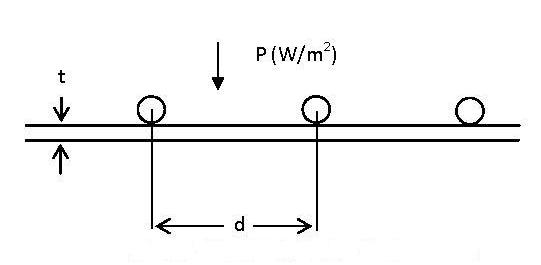 Figure 1. Heat Shield with Cooling Coils
Editors Note:
A few weeks ago Ed Bonnema had a conversation regarding cryomodule design with a potential customer. The conversation roamed over a range of topics from vacuum vessel design, balancing good vacuum design practice vs. reducing cost, etc. One topic of much interest was the design and cost trade-offs between copper and aluminum shields. The customer seemed satisfied with my comments but I felt my answers addressed general concepts without getting into the specifics deep enough. So, Mike Seely and I discussed authoring a newsletter article on the subject. This is the result. Chris and others, I hope this gives you more specific guidelines for decision-making.
I. Heat Shields at 80K
We present some design guides for heat shields. Heat shields are often cylindrical in shape and are cooled either by coils or by attachment to a cold surface at one end. Calculating the temperature profile along the shield then reduces to a problem of heat conduction in one dimension. We start by considering a heat shield of thickness t with a regular array of cooling coils attached at a distance interval d. This could be a cylindrical heat shield with cooling lines run along its length or with cooling lines run around its perimeter. We assume that these cooling coils are attached continuously along their length and fix the shield temperature at 80K along the point of attachment. If the surface is well insulated and in a good vacuum, then the heat flux from a 300K surface is typically 1.0 W/m2. With a uniform heat flux P on the surface, the temperature will reach a maximum value half way between the cooling coils.
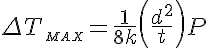
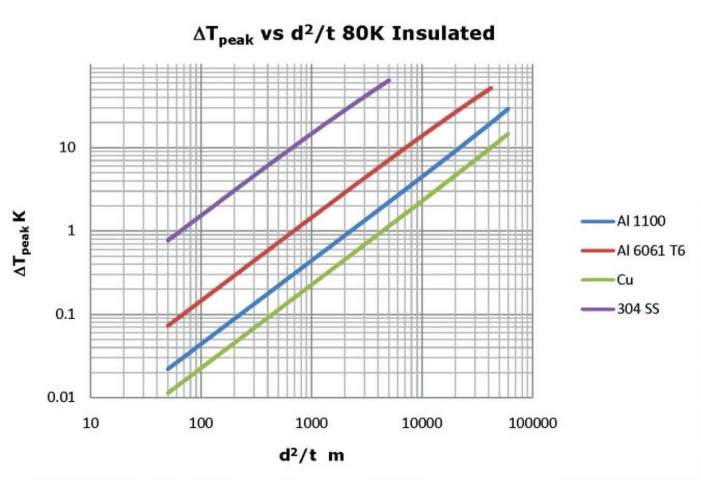 Figure 2. Peak Temperature Rise for Various Shield Materials, Insulated 80K Surface
Where κ is the thermal conductivity of the shield material, the peak temperature scales as d2/t. The results for a number of common shield materials are shown in Figure 2. The thermal conductivity for RRR=300 copper has been used here; however, in this temperature range the thermal conductivity of copper is not highly sensitive to composition and temper. For example, if we have a copper heat shield 0.001m (1mm) thick and coils spaced every 1m then d2/t = 1000 m and the peak temperature rise between the cooling coils is only about 0.2K. The same heat shield would have a temperature rise of about 1.3 K if it were fabricated from 6061T-6 aluminum and about 13 K if it were fabricated from stainless steel. If the surfaces were uninsulated, then the radiated heat flux from a 300K surface would be approximately 90 W/m2 assuming a moderately low value of ε ~ 0.2 for the emissivity. This has the effect of pushing the curves higher ΔT.
In both figures 2 and 3 the value of κ at the average temperature is used to calculate ΔT. The curves are accurate to a few percent at the higher values of ΔT.
In both figures 2 and 3 the value of κ at the average temperature is used to calculate ΔT. The curves are accurate to a few percent at the higher values of ΔT.
 Figure 3. Peak Temperature Rise for Various Shield Materials, uninsulated 80K surface.
Frequently a heat shield design problem will specify a maximum value of ΔT and it is up to the designer to balance issues of cost and ease of fabrication. For example, suppose that we have an insulated 80K cylindrical heat shield and the temperature rise is to be no more than 10K. From Figure 1 we find that a 304 stainless steel heat shield would require d2/t = 650 m, which could be achieved with a 1 mm thick shield with a coil spacing of 80 cm. To obtain the same ΔT with 6061 Al we would require d2/t = 7000 m, which for a 1 mm thick shield would require a coil spacing of 2.6 m. Using 1100 Al for this heat shield would require d/t2 = 21000 m, which for a 1 mm thick shield would require a coil spacing of 4.6 m. Finally, using copper would require d2/t = 41000 m, which would allow a coil spacing of 6.4 m for a 1mm thick shield.
The peak temperature ΔTpeak scales as d2 because increasing d has two effects; it increases the distance over which heat must be conducted and it increases the area per coil and thus the radiated power per coil. Designers often specify a maximum peak temperature that is to be achieved over a heat shield. If an inner 4K surface is being shielded, then it is the average temperature of the 80K shield that is of interest. For this simple geometry the temperature varies quadratically with distance to the coil. The average temperature is:
The peak temperature ΔTpeak scales as d2 because increasing d has two effects; it increases the distance over which heat must be conducted and it increases the area per coil and thus the radiated power per coil. Designers often specify a maximum peak temperature that is to be achieved over a heat shield. If an inner 4K surface is being shielded, then it is the average temperature of the 80K shield that is of interest. For this simple geometry the temperature varies quadratically with distance to the coil. The average temperature is:
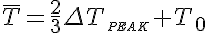
One might wonder if the average value of T4 rather than the average value of T would be the quantity of interest. Thick MLI blankets are normally characterized by an effective conductivity because conduction through the blanket, rather than radiation, becomes the major source of heat flux to the cold surface. In this case it is the average temperature that will be required. For example, assume that we have a 6061 Al heat shield 0.5mm thick with 80K cooling coils spaced every 3 m. With d2/t = 18000 m we would predict ΔT=24K from figure 2. The average temperature of the shield is 80K + 24K(2/3) =96K. The heat flux from a 77K shield to a 4K shield is typically assumed to be 0.07 W/m2corresponding to a thermal conductance of 9.6 x 10⁻⁴ W/m2. In this case we would predict a heat flux of:

In this case, what might appear to be a significant temperature excursion on the 80K heat shield results in an increase in heat flux to the 4K surface that is probably within the uncertainty in our assumed thermal conductance.
The curves above can also be applied to the case of a cylindrical heat shield with one end fixed at T0 ~ 80K by substituting the length of the cylinder for d/2 in Figure 1. The base of the cylinder is being neglected, however, this could be compensated for with reasonable accuracy by adding one half the radius to the length. For example, suppose we have a heat shield which is 1m long, 1m in diameter and 2mm thick made of 1100 Al. This yields (2L)2/t = 2000 m and ΔT ~ 0.9K if the cylinder is insulated. If we wish to take the base of the cylinder into account then the length would be taken as 1.25m and ΔT is then the temperature drop from the center of the base. This approach will tend to overestimate ΔT.
II. Heat Shields at 4K
Figure 4. Heat Shield Characteristics at 4K
The same considerations apply to heat shields at 4K. However, the thermal conductivities and heat load are quite different. Figure 4 illustrates the same case as Figure 2 but at 4K. The thermal conductivity of copper used here corresponds to C101 with an RRR of 150. This corresponds to a relatively soft form of C101 with little cold working. At these temperatures the thermal conductivity of copper varies considerably depending on the purity and temper.
Real heat shields rarely have perfect cylindrical symmetry and it is not always possible to place cooling coils at perfectly regular intervals. Simplifying a real heat shield to a heat conduction problem in 1 dimension is an approximation. At the same time, our knowledge of the thermal conductivities is often only approximate. Their values are generally affected by cold working, which is difficult to quantify. Our knowledge of the effective thermal conductance of MLI is also imperfect. The approximations made in simplifying the heat shield geometry are not unreasonable in view of other approximations made in heat shield design. Our approach would generally be to make the design contingency sufficiently robust to insure that the heat shield meets specification in spite of the approximations made.
III. Conclusions
- Stainless steel has been included in the design charts, although it is not frequently used as a heat shield. It is necessary to use a thicker shell and/or more closely spaced cooling coils to match the thermal performance of an aluminum or copper heat shield using stainless steel. However, the ease of fabrication may favor stainless steel in some applications.
- At 80K the thermal characteristics of copper and aluminum do not vary greatly. Similar thermal performance can be obtained by varying the thickness of the shield. The differences are greater at 4K.
- The thickness of the shield and the spacing of cooling coils can be varied to obtain similar thermal performance from different materials. Considerations such as weight, cost and ease of fabrication may then favor one material over another.
- The peak temperature between the cooling coils scales as d2/t. Doubling the coil spacing increases the peak ΔT by a factor of four, while cutting the thickness in half increases the peak ΔT by a factor of two.